*Sed ut perspiciatis unde omnis iste natus error sit voluptatem accusantium
Quantum neural networks | Effortless reading
Amitnikhade
July 1, 2021
We gonna explore Quantum neural networks (QNN) in a much simplified manner, covering all the fundamentals concepts that will create a grasping impact. I’ll try making you understand with least mathematics to get a better overview as a beginner.
Introduction
Artificial Neural Networks (ANN) has been a generous algorithm on which the whole deep learning field is footing steady. ANN consists of the collection of neurons connected with each other. each neuron in the network can share information with each other using connections, which in terms of biology are called synapses of the biological neurons in the brain. Nowadays lots of new models are built on top of neural network architecture with state of art performance.
A quick overview of ANN’s
ANN consists of interconnected group neurons, passing information to each other. The ANN is an idea inspired by the human brain mechanism, which also poses a behavior similar to artificial neural networks. In the figure below the circular nodes represents the artificial neurons. And the arrows are the connections to pass information from one neuron to another. The deep neural network contains an input layer, hidden layers, and an output layer. The hidden layers are the fully connected layers with all possible connection scenarios. Let us move forward with some fundamental terminologies concerning the Artificial neural network. I won’t go into the much deeper section. hoping you are familiar with the Neural network and deep learning.
- Neurons: The neuron is the node that involves some mathematical operation. When the input is passed to it, It multiplies the input by the weight and the output is passed to other neurons through the activation function.
- Connections: The connections are the medium of passing information between the neurons.
- Weights: The weight is one of the learnable parameters of an ANN model. it decides how much influence the input will have on the output. it transforms the data fed to it, within the network’s hidden layers. It tells the strength of the connection between neurons.
- Feed-forward networks: The elementary neural network in which the information moves only in one direction i.e the forward direction. It is a loopless network
- Recurrent neural network: The RNN’s recurrent neural network is a variant of the vanilla neural network which was created to remember or memorize information using the hidden layers that helps remembering information about a sequence. It allows the reuse of previous output as an input. Some applications of Recurrent neural networks are neural machine translations, chatbots, sentiment analysis, etc.
- Convolutional neural networks: The Convolutional neural network was specifically designed to process pixel data. Mainly, it focuses on image data. Where multiplying pixel values by weights and summing them up is called convolution. Applications of convolutional neural networks are object detection, image classification, etc.
- Backpropagation: Backward propagation is the opposite of the feed-forward, where the backward pass is performed by adjusting the trainable parameters. Back Propagation uses the chain rule to perform the backpropagation. In simple terms, the backpropagation computes the gradient of the loss function with respect to the weights.
To understand the quantum neural network part, you need to understand the neural network basics and its working. So without wasting much time on the classical neural networks, let’s put focus majorly on the quantum neural networks.
I have been separately created articles on the basics of Quantum machine learning, Please read them before proceeding further.
On this current site amitnikhade.com and on Medium @amitnikhade
Introduction to Quantum neural networks
One of the major differences between quantum and classical neural networks is parallel computation. The quantum neural networks are similar to classical neural networks excluding some changes. They serve as the newer class in Quantum machine learning. This model is deployed on Quantum computers and makes use of quantum properties like superposition, interference, entanglement to perform computations. Their major advantages include accelerated training and processing. QNN’s are the subclass of variational quantum algorithms.
The Quantum neural networks comprise the quantum circuit consisting of parameterized gate operations.
Steps involved
To begin with, the inputs are first encoded to quantum states, however, in classical computing, we do the same which is called embedding the input before feeding to the network. The encoding is done using a feature map, which I have briefly explained in my last post on quantum embedding. In addition, the encodings are passed to the variational model consisting of parameterized gates, and the model is optimized for a particular task by minimizing the loss. In conclusion, the measurements are done and we get an output.
let’s go a bit deeper into the above steps
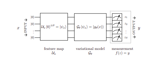
A Quantum neural network is used to refer to variational or parameterized quantum circuits. The replacement of the perceptron in the Quantum neural network is the Qubit which reduces the size of parameters. This time we will consider the above diagram. which comprises a feature map, a variational model, and measurement. where x inputs are into classical data form which first has to be embedded into quantum states in the Hilbert space using the feature map. The state preparation process allows encoding of the input data onto qubits as a quantum state in superposition. The encoding can be different types, I already have explained them in my previous posts, you can visit them on my website. The qubits are now entangled in such a way that modification of one state influences the state of others. furthermost, they are fed to the variational model i.e the quantum variational circuit that is composed of series of parameterized gates like RY-gates for the rotation and CNOT for entanglement. And lastly, the Post-processing step performs measurements, which measure the parity of the output. The parameters of the rotations are modified until and unless the circuit gets the desired result. The measurement itself acts as an activation function.
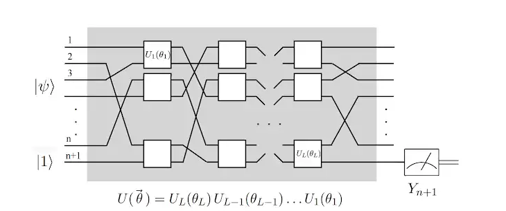
In the figure, where |ψ〉 is the desired state, |1〉 is the readout qubit, Yn+1 is the measured value. The Boxes in the networks are the quantum gates that change the states of the initialized qubit with parameters that are simultaneously and eventually changed.
The inputs are encoded into states and the qubits are initialized at state |0〉. As the states flow through the circuits the states of qubits are changed.

Assuming the qubit states to be initialized, we perform the unitary transformation Ui(θi) that depends on parameters θi. These get adjusted during learning such that the measurement of Yn+1 on the readout qubit tends to produce the desired label for |ψi. A matrix is said to be unitary only if the inverse of the matrix is equal to its adjoint.
Implementation
Let’s try coding the QNN in Python.

We’ll need Tensorflow Quantum installed.
Here are the installation steps. You’ll need Python 3 installed.
Firstly we’ll create a python environment.
conda create -n ENV_NAME python=3
Next, we’ll activate it.
conda activate ENV_NAME
Furthermost, we’ll install the TensorFlow v2.4.1package
pip3 install --upgrade pippip3 install tensorflow==2.4.1
Finally, install the TensorFlow Quantum package
pip3 install -U tensorflow-quantumImport Packages
import numpy as np
import matplotlib.pyplot as plt
import tensorflow_quantum as tfq
import tensorflow as tf
import cirq
import sympy
import random
Create a qubit
Here we have used Grid Qubits, The GridQubits have a row and column, indicating their position on a grid.
qubit = cirq.GridQubit(0,0)
Create train test
Creating separate lists for appending train and test split.
train, test = [], []
train_label, test_label = [], []
Data Preparation
Making data ready by Encoding data as a quantum circuit, splitting them into train and test data, converting them to tensors, and appending them to the list we created at the starting.
Create a circuit
The circuit is composed of gates operations to perform rotations on qubits.
Define accuracy function
hinge_accuracy metric can handles [-1, 1] rightly.
Create model readout
Plot circuit

Create a hybrid quantum model
We would create the input, output layers. Converting the circuit into a Tensorflow quantum layer and define the measurement operator which we would optimize. Using the Parameterized quantum circuit layer with parameter shift differentiator. Typically the measurement is not certain. Our predicted value is the real number between −1 and 1. The parameterized quantum circuit is a quantum circuit that can freely adjust its parameters. Model is compiled using Adam optimizer and hinge loss. The Differentiator class allows you to define algorithms for computing the gradients of your circuits.

For the hinge loss here you need the data in [-1, 1], as expected by the hinge loss as well as it needs hinge accuracy.
Training Time
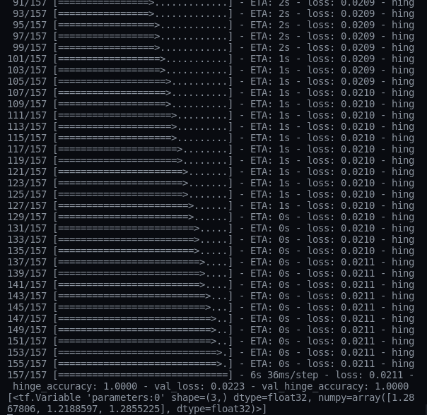
Performance
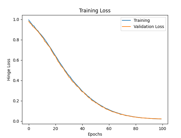
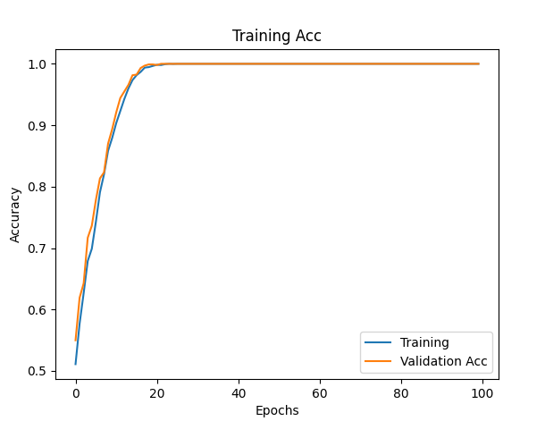
Great you have reached the destination. Hope you enjoyed the explanation which I tried making theoretical majorly for it to be understandable.
Conclusion
Even today, Quantum computing hasn’t qualified the operation and computing tasks we want it to do. Classical machine learning is outperformed by Quantum machine learning but not in all terms and problems. We need much more advancements to reach the quantum level as it can yield wonders in technology. Quantum computing poses the power to transform the imaginary world into reality if used accordingly.
Do not forget to hit claps and follow me on medium.com, if you found the writings insightful.
Originally Published on amitnikhade.com
References
These references helped me a lot, also go through them.
https://arxiv.org/abs/1802.06002
https://ai.googleblog.com/2018/12/exploring-quantum-neural-networks.html
https://quantumai.google/cirq/tutorials/variational_algorithm