Logistic regression (Lucid Explanation)

Let’s understand the logistic regression without any elaboration and in a short manner, that won’t waste your time rather than it will deliver you just the needed information. So don’t even have a cup of coffee with you, before sipping the coffee you’ll grasp logistic regression.

Introduction

Logistic regression is the foundational algorithm essential for moving forward in streams like machine learning, deep learning, data science, etc. It’s a simple model, but a bit confusing, if you know the linear regression model.

“Educate, agitate and organise. Have faith in yourself. ”

-Dr. B.R. Ambedkar

Note: Before you go through this article, I hope that you at least know the basic working of Linear Regression. If not I recommend you to please go through this article once. I bet you’ll get all of it. All the best.

Logistic regression at a glance

Logistic regression( maximum entropy model or logit regression model), a statistical model also implemented in machine learning as a logistic regression model, supervised Machine Learning algorithm used for classification tasks that uses a logistic function to classify the binary data. The Logistic function is nothing but the Sigmoid function that we’ll be seeing further. It is also used in various other fields including Machine learning. It simply separates data into the categories they belong to. It is used when the target variable is categorical (having two or more categories of data). The Binary logistic model can categorize data into two types. And the model that can handle data with more than two types (classes) is called multinominal logistic regression (polytomous, polychotomous, multi-class logistic regression, multi logit regression). The regression model can handle ordered data, having more than two categories like Ordinal Logistic Regression, but in the case of multinominal, the data is orderless.

let’s not get confused between the logistic and the linear regression

Let’s see how logistic regression meets linear regression. The only major factor that differentiates both the methods is the way of delivering the output, where the linear regression uses a linear plane to predict the data, on the other hand, the logistic regression uses the curve that looks S shape also called the logistic function or sigmoid. The output of logistic regression is discrete and that of the linear regression is continuous. both the models (Linear Regression and Logistic Regression) are parametric i.e. both use linear equations for predictions.

Why not linear regression?

There are mainly two reasons why linear regression can’t be used for a classification problem. Linear regression can classify data but only if there is no outlier and the data is not extended beyond the threshold limitations required for the classification, I hope you didn’t understand what exactly I mean. Let’s take a brief and simple overview.

Outlier effect: The outlier is one of the major factors responsible for incorrect classification results using linear regression. Suppose we have data points plotted on a graph as given below, and we fit a line to classify the values, whether they are infected or not (green line). In the case of the green line, we can see that the values are classified properly, but as soon as we add an outlier the green line is changed to red line and our results got changed completely, due to one value all have to face.

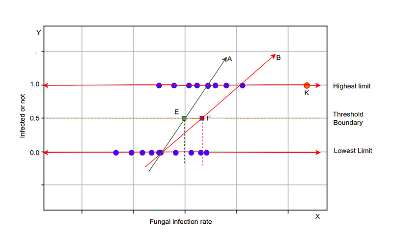
As we can see how the performance is affected due to the sudden change in the best fit line due to an outlier. An outlier increases the error rate in the results

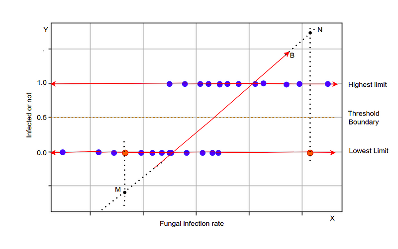
Value overflowed: If the plane of the regression exceeds the limit of the threshold due to a bigger x value. So in this case what shall we consider? To overcome this problem we need to convert it into a certain range so that it won’t exceed the limit.

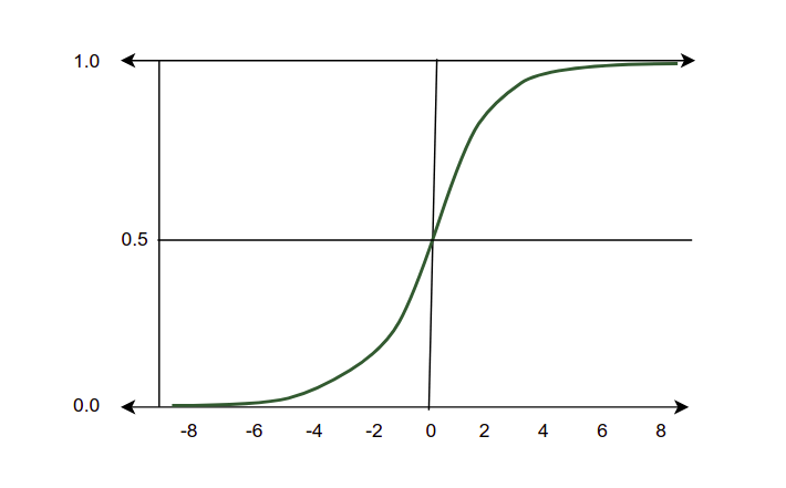
Sigmoid

Sigmoid is an S-shaped curve that transforms values from range 0 to 1, also known as logistic function. As we know we are discussing the classification algorithm so we are expecting output as a discrete value either 1 or 0. but In the case of linear regression when we try to separate the data points with the line we get continuous values that can be below zero as well as above 1 or floating values, that isn’t what we need. So to overcome this problem and to get a clear output in binary form, we need the sigmoid function that scales the values between 0 and 1. If the value is greater than 0.5 we consider it as one and if it’s less than 0.5 we consider it as 0. And hence we get a crystal clear output.

                     

Note: e is the Number of Euler. x is the value passed to the equation.

In Python, the sigmoid is coded as

                      sigmoid = 1 / (1 + e**(-z))

you may get confused between log odds and sigmoid, let me tell you, both the terms are the same, but a question occurs, what is odds?

The odd is defined as the probability of an event occurring divided by the probability of the event not occurring.

                                                                 

 

 

Cost function

 

 

The cost function is used to evaluate the performance of the model. But as we saw in linear regression we use mean square error as the cost function but in the case of logistic regression, we can’t use the same. But why?

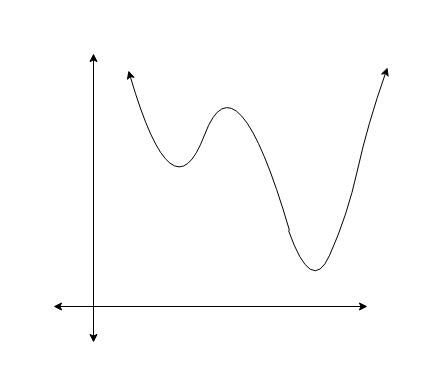
The MSE cost function can’t be used as the loss function for logistic regression this is because we know that logistic regression is a non-linear model which is due to the sigmoid function. The z value(sigmoid) in the code implementation is non-linear function. Now just think that if we use the z value in the MSE loss function we get a non-convex curve as shown below

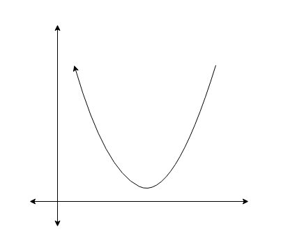
but for performing gradient descent optimization we need the curve given below, which makes it easy to reach the global minima. But in the case of the above curve, it will go through complications to reach the global minima and won’t give the desired performance as it will result in non-convex function with many global minimums. The required curve for gradient descent is as shown below.

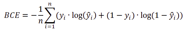
So we use a cost function called Cross-Entropy, also known as Log Loss for logistic regression. Cross-entropy is a simple cost function with some basic calculations. The step involved in calculating cross-entropy is as follows:

1. Calculating the corrected probabilities.
2. Calculating log of corrected probabilities.
3. Calculate the negative average of the obtained values.

In the first step, we have calculated the corrected probabilities. The corrected probabilities are nothing but the value obtained by deducting the predicted probability value from one, this is done if the actual target is zero and the predicted probability value is greater than zero. This is not applied when the target is one. You just need to keep these steps in mind.

Next, we need to take the log of the corrected probabilities.

                           

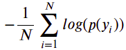
And further, we need to take out the overall negative average of the resulting value

                           

 

 

 

Maximum likelihood

                               

 

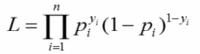
As we know that we can’t use the least Square here, for logistic regression we need something called likelihood. Maximum likelihood is like an optimization problem that helps us in finding the parameters of the model in such a way that it calculates the product of the probabilities and the rule is that the product should be maximum, let’s see what this means?

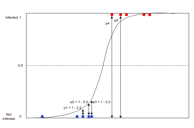
In the above diagram, we can see the probabilities p1, p2, p3, p4, and p5. The probability of not infected points are, as shown above, they are calculated by deducting the length (from the value from the x-axis to the sigmoid curve) from 1. Even if the blue dot lies above 0.5 the same procedure is applied to calculate the probabilities. And for the redpoint, the probability is measured as the distance from the x-axis to the redpoint.

Let take an instance and focus on what is exactly happening.

                                                                                                                                                                                                                                                                                                                 table

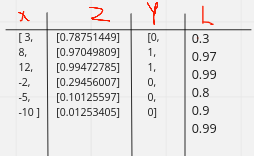
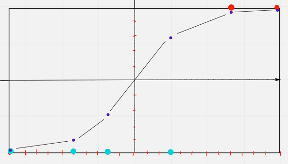
As we can see in the table, we have x values plotted on the graph below according to their targets (0, 1). After converting the values in range 0 to 1 using sigmoid we get the z column and the s curve in the graph. Further, we calculate the likelihood of all the values.

 

                                                            

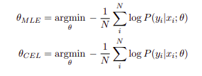
likelihood modified with log and negative sign,  So maximum likelihood in sense will get the least as possible because we have applied negative sign to it.

 

Don’t get confused between the maximum-likelihood and cross-entropy

I know you might be getting confused between the ML and CE. But that is almost the same if we take the negative log of the likelihood, we get the cross-entropy cost function. maximizing the negative log-likelihood is equivalent to minimizing the cross-entropy. So no difference existed between the two functions.

 

 

                                

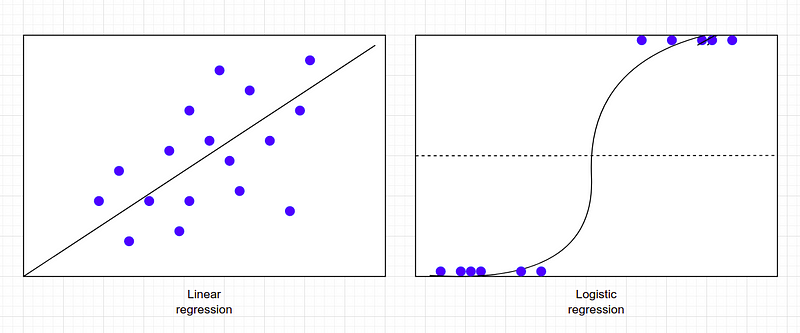
Linear regression predicts continuous values whereas logistic regression predicts discrete values. Linear regression solves regression problems whereas logistic regression solves classification problems. Linear regression uses a straight line to predict values whereas the logistic model uses a sigmoid s shape curve to classify values.

Working

Being familiar with linear regression is a must to understand the working of logistic regression. The logistic regression has a simple working mechanism, which we will be understanding by a simple example.

Let’s consider a dataset having two columns with a target column. The dataset is a classification problem where the target specifies whether the person is infected or not.

Here is the algorithm:

Step 1:Firstly we’ll convert the data points in the range 1 to 0 using a sigmoid function.

Step 2:Next will calculate the weight and update them. 

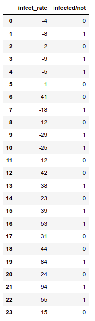
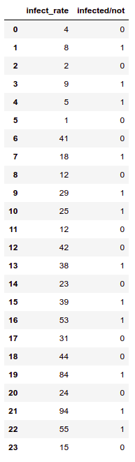
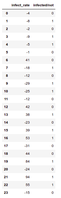
Let’s consider an instance where the below data has two features and one target. Our task is to classify whether a person is infected or not. The label consists of labels 0 and 1, where 0 indicates not infected and 1 means infected.

                                                  

Let’s take a row where

x = [-4,-8,-2,-9,-5,-1,41,-18,-12,-29,-25,-12,42,38,-23,39,53,-31,44,84,-24,94,55,-15], y = [0,1,0,1,1,0,0,1,0,1,1,0,0,1,0,1,1,0,0,1,0,1,1,0].

By passing the x values from the sigmoid function we get a curve something like this

and the outputs are sigmoid:

[6.81859658e-02 5.32613544e-03 2.12914325e-01 2.77725088e-03
 3.66636042e-02 3.42150918e-01 1.00000000e+00 7.75608400e-06
 3.91676137e-04 5.84321251e-09 7.98520186e-08 3.91676137e-04
 1.00000000e+00 1.00000000e+00 2.95190877e-07 1.00000000e+00
 1.00000000e+00 1.58064579e-09 1.00000000e+00 1.00000000e+00
 1.53530417e-07 1.00000000e+00 1.00000000e+00 5.51248752e-05]

As we can see the values are above 1, but the sigmoid output should range between 0 to 1. the reason why we got values above 1 is that we have negative x values.

If we convert the value to positives and pass them from the sigmoid

                                                  

we get a curve that appears something like this

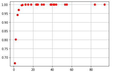
and output of sigmoid are :

[0.77124819 0.91914194 0.64741284 0.93903704 0.82042297 0.57538174
 0.99999611 0.99580299 0.97457127 0.99985101 0.99949783 0.97457127
 0.99999713 0.99999033 0.99907832 0.99999286 0.9999999 0.99991885
 0.99999844 1. 0.99931966 1. 0.99999994 0.98962213]

Now you might notice that the value is in the proper range.

σ(x) = 1/(1+exp(-x))

There is also a weight parameter that is multiplied with the data. The initial value of weight is randomly defined and get updated on each iteration. Assume, that our random weight(w) was 0.30133235

σ(x) = 1/(1+exp(-x.w))

using the above equation each value of x is converted between 0 to 1.

Step3: Gradient

Next, we will calculate the gradient i.e we will calculate new weights (updating weights). Gradient descent is an iterative optimization algorithm that simply is used to update parameters in such a way that the loss of the model must be the least. For that, we need to first define the learning rate, the learning rate is the hyperparameter that determines the step size at each iteration while moving toward the global minima. A too-small learning rate value may result in a long training process that could get stuck, whereas a large one may result in an unstable training process where the model finds it difficult to get converge. If you have gone through the previous linear regression article you may understand this very well, no doubt.

                                           

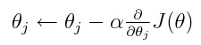
The above equation is the gradient descent, where alpha is the learning rate multiplied by the partial derivative of the cost function.

where

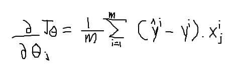
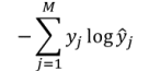
In this equation of the cost function y_hat is the sigmoid output and y is the target value.

In python, the gradient optimizer equation can be coded as

weights -= lr * dot(X.T,  y_hat - y) / N

If you won’t understand the translation from the equation to the code, try to understand yourself. Just not being rude, but advising a good habit.

Next, we’ll be applying several iterations on the same algorithm until and unless we don’t find the best parameters and after getting some good parameters we’ll get to see classification results with awful results.

Github

Implementation

from numpy import log, dot, e
from numpy.random import rand

class LogisticRegression:
    
    def sigmoid(self, z): 
        return 1 / (1 + e**(-z))
    
    def cost_function(self, X, y, weights):                 
        z = dot(X, weights)
        predict_1 = y * log(self.sigmoid(z))
        predict_0 = (1 - y) * log(1 - self.sigmoid(z))
        return -sum(predict_1 + predict_0) / len(X)
    
    def fit(self, X, y, epochs=25, lr=0.05):        
        loss = []
        weights = rand(X.shape[1])
        N = len(X)
                 
        for _ in range(epochs):

            #passing x values through sigmoid and calculating 

the gradient         
            y_hat = self.sigmoid(dot(X, weights))
            weights -= lr * dot(X.T,  y_hat - y) / N            
          
            loss.append(self.cost_function(X, y, weights))

        #updating weights    
        self.weights = weights
        self.loss = loss
    
    def predict(self, X):        
        
        z = dot(X, self.weights)
        
        return [1 if i > 0.5 else 0 for i in self.sigmoid(z)]

Let’s see this in action

# our data

df = pd.DataFrame({'infect_rate':[-4,-8,-2,-9,-5,-1,41,-18,-12,
-29,-25,-12,42,38,-23,39,53,-31,44,84,-24,94,55,-15], 'infected/not'
:[0,1,0,1,1,0,0,1,0,1,1,0,0,1,0,1,1,0,0,1,0,1,1,0]})

                                                    

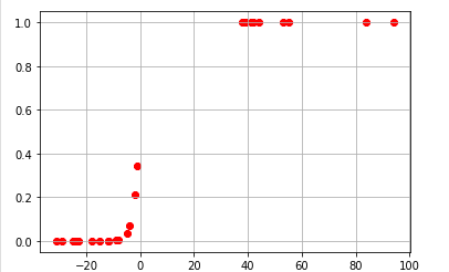
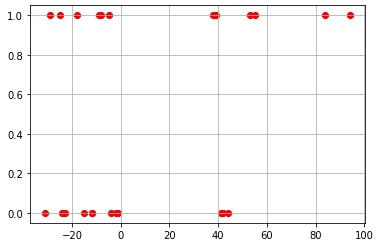
x = np.array(df.infect_rate).reshape(24,1)
y = np.array(df['infected/not']).reshape(24)

plt.scatter(x,y, c = 'red',cmap='viridis')
plt.grid()
plt.show()

L = LogisticRegression()
L.fit(x,y)

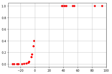
if we try plotting sigmoid we get

plt.scatter(X,y_hat, c = 'red',cmap='viridis')
plt.grid()
plt.show()

test = np.array([39]).reshape(1,1)
L.predict(test)

output:
[1]

Conclusion

It’s not the case of understanding the mathematics, but just the concept can automatically help you in deriving the equations. Logistic regression can’t handle a large number of features. Logistic regression had many more extensions like multinomial logistic regression, conditional logistic regression, ordered logistic regression, and many more, we’ll be seeing them in future meets.

References

I have referred to multiple sources to understand logistic regression when I started the journey because a single source can’t explain everything, even I must have missed some concepts, if you noticed some please comment below.

medium, google, Wikipedia, arxiv, and multiple sources.