Entropy and Information gain

Photo by Kyle Roxas Some moments occur when we notice that we have seen this term somewhere and we don’t remember what it exactly means. Entropy and information gain belong to the same categories of terminologies.

We will try to understand entropy and information gain in a very simple and uncomplicated way. A basic understanding of the decision tree is required to understand these two terminologies. If you haven’t yet seen what is a decision tree, that really cool you are at the right address, you’ll take away something memorable from here.

Decision tree at a glance

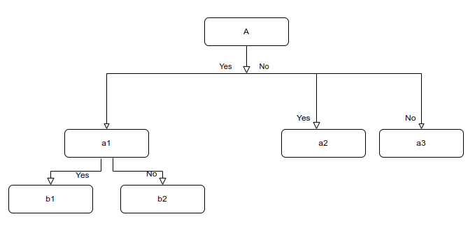
A tree-like structure that flows from top to bottom like a flowchart. A supervised learning method is used for both classification and regression problems. As shown below. The components of a decision tree consist of a node that represents a feature(attribute), The branch represents a rule or condition and each leaf represents an outcome that can be into a categorical or continuous value form.

The methods that are used to build the decision tree are basically the CART(Classification and Regression Trees) and ID3(Iterative Dichotomiser 3). In our case, we’ll be diving into the ID3 method that includes entropy and information gain techniques.

                                                     

Let’s take a look at the working of the decision tree quickly. Now consider an instance where we have a dataset consisting of 2 features height and weight. And the labels are whether the person has a fit or unfit body type. It’s a classification problem.

                                                                                                                       

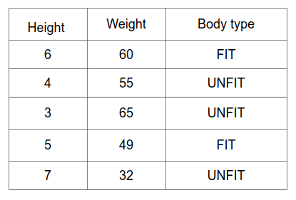
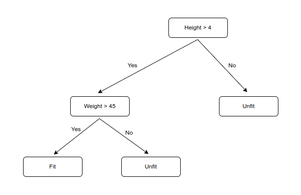
In the table, we can see how the labels are classified according to height and weight. The root node and the intermediate node represent the features of the dataset and the leaf node represents the labels. In the figure, the root node is split into two branches where if the condition height greater than four is true then we further split the node as per the second condition where the weight has to be considered above 45. If the first condition is false the splitting is stopped. In the second condition having a weight above 45 is true we consider the person as fit else if the condition is false we consider it as an unfit body. When a person meets both the conditions, he/she is said to be fit, else if it does not meets any one of the condition, then the person is said to be unfit.

                                                             

Now, You might be wondering how exactly is the decision tree constructed, and what’s the procedure. In the beginning, we saw how the methods of creating the decision tree, in our case we use the ID3 method as we are dealing with a binary classification problem. Let’s see how exactly it flows.

1. Firstly, we will select the best features to create a node that will split properly. The feature selection is done using top to down greedy approach that is iterating from top to bottom and at each, it selects a feature.
2. For feature selection, the information gain finally comes into role. we’ll come to IG later.
3. Split the data into subsets using the feature having maximum information gain.
4. Construct a node using the feature with the maximum Information gain.
5. If all rows belong to the same class, the node is considered a leaf node. Else the node is split.
6. The interaction goes on until and unless all features are not categorized, whether they are eligible for splitting or are leaf nodes.

Information Gain

Information gain is the measure of the information given by a node. where the maximum information providing node is selected, it measures how well a feature classifies the class. In other words, the Information Gain calculates the reduction in the entropy. let us see how the information gain is calculated.

                                             

The information gain is the measure of the difference between the entropy of the parent node and the entropy of the child node that we get after splitting the parent node. In the equation S is the parent node.

A is the features in the data.

S tells the number of data points in the whole dataset.

Sᵥ tells the number of times the value of A occurs while

The Information gained tells how many impurities in S were reduced after splitting it to the subnode.

Entropy

Entropy is the disorder, uncertainty, and impurity in the data. Let us suppose in a data frame of five rows where the labels are the same, the entropy would be zero as it is a pure node having all labels the same, and if the labels have variations then the entropy is one. the entropy ranges from 0 to 1 in the binary classification and in multiclass classification, the entropy is defined as:

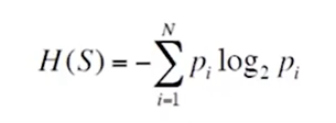
where S is the data. N is the number of classes and pi is the probability of the event i.e the amount of samples that belong to a particular class for a particular node. (number of rows with a particular class in the target column: total number of rows in the dataset)

• If all classes in the dataset are the same then entropy will be zero i.e, low.
• If classes in the dataset are balanced with the same amount of both classes, then entropy is one i.e, high.

Implementation

Firstly we will see how the entropy is calculated. In simple terms we have to just subtract the product of the (- class occurrence/total classes) and log to the base 2 of (- class occurrence/total classes). same with the second class occurrence.

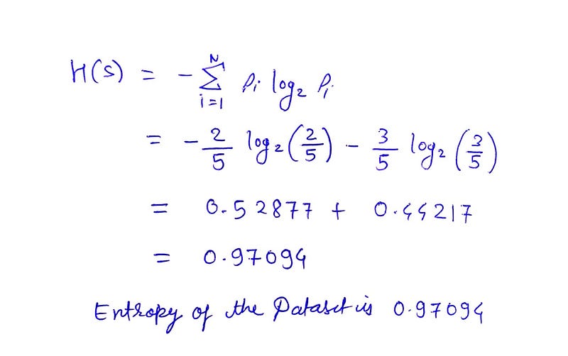
The entropy of our dataset is 0.97094 i.e the impurity.

Let’s split the dataset by data having a weight greater than 45 (w>45). We’ll see how much information is gained after doing the split. For that, we will need to calculate the entropy of the data with the true conditions, as shown below.

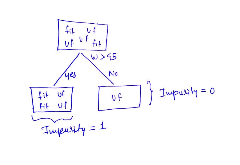
Let’s calculate the entropy of the split data frame (Parent node) as shown above. We know that if the classes are balanced the impurity is 1. And if there is just one cell or the same occurrence of the class, then impurity has to be 0.

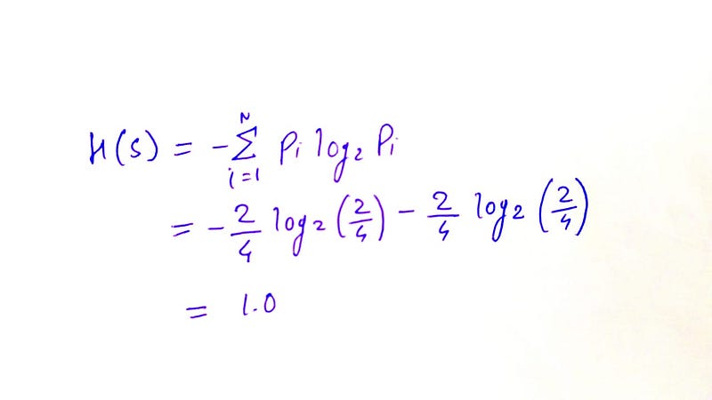
As we have the parent node entropy and the split node entropy we can now move forward with the gain calculation. Gain is the difference between the parent node entropy and the split node entropy.

So, the information gain is 0.71094. The gain should not be negative.

There are other commonly used algorithms to build a decision tree. They are CART (Classification and Regression Trees) — Which makes use of Gini impurity as the metric.

Conclusion

Decision trees are one of the most powerful algorithms of machine learning to perform classification and regression tasks. They take less time to make predictions. Not even the missing value imputation is required. They also pose some cons like they are prone to overfitting that can be overcome using the ensemble methods like the random forest. There are other ML algorithms that outperform decision trees, it totally depends on the type of data suitable for a particular algorithm.