*Sed ut perspiciatis unde omnis iste natus error sit voluptatem accusantium
Hacking an Artificial neural network
Amitnikhade
July 11, 2023

They also have a weak spot — they can be hacked!
Adversarial attacks, where inputs are tweaked to mislead these networks, have become a concern. In this post, we’ll explore the basics of hacking neural networks in a responsible and ethical manner.
What is it?
The FGSM (Fast Gradient Sign Method) is a type of attack that falls under the category of adversarial attacks. Adversarial attacks have become a hot topic in the field of deep learning, much like how information security and cryptography are important in computer science as a whole. Adversarial examples can be thought of as the equivalent of viruses and malware for computers, but in the context of deep learning models.
Some useful terminologies
Adversarial example: Adversarial examples are carefully crafted samples created with the intention of causing machine learning models to make mistakes.
Perturbation: Perturbation refer to small modifications added to the input data to deceive the model’s predictions and exploit vulnerabilities in the model’s decision-making process.
Epsilon: Epsilon is a small number that determines the strength of an adversarial attack. It needs to be selected thoughtfully to make the attack effective without being too noticeable. It is denoted by ϵ.
Assuming that you are aware of the gradient and loss function, if not first go through any blog or video explaining the working of ANN.
How does it work?

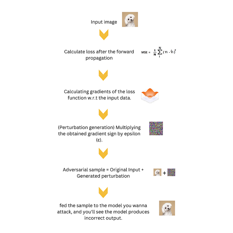
- Input: We start with a pre-trained machine learning model and a specific image that we want to modify to trick the model.
- Compute the gradient: We calculate how sensitive the model’s prediction is to changes in the input image. This is done by looking at how the model’s loss function changes when we make small adjustments to the image.
- Determine the perturbation: We figure out the direction in which we should modify the image to make the model more likely to make a wrong prediction. To do this, we look at the sign (positive or negative) of the gradient we computed earlier.
- Specify the perturbation magnitude: We decide how much we want to modify the image. This is controlled by a parameter called epsilon (ε). A smaller epsilon means a subtle change, while a larger epsilon means a more noticeable alteration.
- Generate adversarial example: Using the gradient sign and the chosen epsilon, we create a perturbation that we’ll add to the original image. This perturbation is calculated by multiplying the gradient sign by the epsilon value.

where
adv_x : Adversarial image.
x : Original input image.
y : Original input label.
ϵ : Multiplier to ensure the perturbations are small.
θ : Model parameters.
J : Loss.
6. Evaluate the adversarial example: We input the altered image (adversarial example), into the model and examine its prediction. The objective is to create an image that closely resembles the original but tricks the model into making an incorrect prediction.
Where is it used?
The FGSM technique is used to create tricky examples that can trick and harm machine learning models. It helps test how strong a model is, find ways to make it more secure by training it against these attacks, study security concerns, and gain a better understanding of how models behave. FGSM is important for making machine learning security better and advancing our knowledge in this field.
How to use it practically?
Here is the python Implementation of FGSM.
We’ll start with training the MNIST image classifier.
import numpy as np
import tensorflow as tf
from tensorflow.keras.datasets import mnist
from tensorflow.keras.models import Sequential
from tensorflow.keras.layers import Dense, Flatten
# Load MNIST dataset
(x_train, y_train), (x_test, y_test) = mnist.load_data()
# Normalize pixel values
x_train = x_train / 255.0
x_test = x_test / 255.0
# Convert labels to one-hot encoding
y_train = tf.keras.utils.to_categorical(y_train, 10)
y_test = tf.keras.utils.to_categorical(y_test, 10)
# Create a simple feed-forward neural network model
model = Sequential([
    Flatten(input_shape=(28, 28)),
    Dense(128, activation='relu'),
    Dense(10, activation='softmax')
])
# Compile the model
model.compile(optimizer='adam',
              loss='categorical_crossentropy',
              metrics=['accuracy'])
# Train the model
model.fit(x_train, y_train, epochs=5, batch_size=32, validation_data=(x_test, y_test))
Next we’ll Apply the FGSM.
import matplotlib.pyplot as plt
def fgsm_attack(model, x, y_true, epsilon=0.9):
    # Compute gradients of the loss w.r.t. the input
    with tf.GradientTape() as tape:
        tape.watch(x)
        predictions = model(x)
        loss = tf.keras.losses.categorical_crossentropy(y_true, predictions)
    gradients = tape.gradient(loss, x)
    # Get the sign of the gradients
    gradients_sign = tf.sign(gradients)
    # Generate adversarial examples
    x_adv = x + epsilon * gradients_sign
return x_adv
# Select a random test sample
index = np.random.randint(0, len(x_test))
x_sample = x_test[index].reshape(1, 28, 28)
y_true = y_test[index].reshape(1, 10)  # Reshape y_true to (1, 10)
# Convert x_sample to a TensorFlow tensor
x_sample = tf.convert_to_tensor(x_sample, dtype=tf.float32)
# Generate adversarial example using FGSM attack
x_adv = fgsm_attack(model, x_sample, y_true, epsilon=0.1)
# Predict the label for the original and adversarial example
y_pred_original = np.argmax(model.predict(x_sample), axis=-1)
y_pred_adv = np.argmax(model.predict(x_adv), axis=-1)
# Plot the original and adversarial images
plt.figure(figsize=(8, 4))
plt.subplot(1, 2, 1)
plt.imshow(x_sample.numpy().reshape(28, 28), cmap='gray')
plt.title(f'Original Image\nPredicted label: {y_pred_original[0]}, True label: {np.argmax(y_true)}')
plt.axis('off')
plt.subplot(1, 2, 2)
plt.imshow(x_adv.numpy().reshape(28, 28), cmap='gray')
plt.title(f'Adversarial Image\nPredicted label: {y_pred_adv[0]}, True label: {np.argmax(y_true)}')
plt.axis('off')
plt.tight_layout()
plt.show()
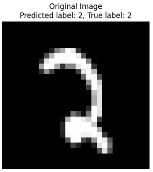
Outcomes from the original image. The Image got classified accurately.

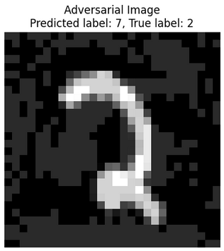
Outcomes with the adversarial example, the TensorFlow model was fooled successfully.

Here is the link to complete code.
Typically, the adversarial image and the original image should appear similar to each other in order to be undetectable by humans, yet capable of triggering a response from a neural network. In my situation, the images can be distinguished from each other because the adjustment of the epsilon value was not executed correctly. However, during the attack, the effectiveness depends on staying within the epsilon range that makes the images look similar.
To sum it up, we’ve covered the basics of the FGSM attack, which helps us understand how it works. By tweaking an image using gradients, we can create deceptive versions that fool neural networks while appearing almost identical to the original. It’s important to know that this field is constantly advancing, with new techniques and strategies being developed. To stay updated and navigate the challenges of adversarial attacks, it’s crucial to keep learning and exploring. By doing so, we can contribute to building more secure AI systems that can withstand these manipulations.
Thanks.
Here’s my LinkedIn
I reside at amitnikhade.com
References:
Explaining and Harnessing Adversarial Examples
Several machine learning models, including neural networks, consistently misclassify adversarial examples — -inputs…arxiv.org
https://engineering.purdue.edu/ChanGroup/ECE595/files/chapter3.pdf
https://adversarial-ml-tutorial.org/adversarial_examples/

