*Sed ut perspiciatis unde omnis iste natus error sit voluptatem accusantium
LCN-An Experimental initiative
Amitnikhade
June 22, 2024

Time-traveling algorithms sipping coffee, predicting the future. But wait, there’s a new kid on the block — the Liquid Capsule Network for Time Series Forecasting (LCN-TSF). It’s like James Bond meets data science, decoding tricky patterns. Buckle up, because we’re diving into LCN-TSF’s secret lair!
Meet the LCN-TSF
The LCN-TSF model is built with some advanced but cool components:
- Liquid State Machine (LSM): Think of it as a neural network with a splash of chaos, perfect for handling tricky temporal patterns.
- Capsule Networks: These preserve spatial hierarchies and dynamic routing, making sure we capture all the juicy details in the data.
- LSTM-based Decoder: An LSTM layer that decodes the processed data and makes predictions.
What motivated me
I’m driven by curiosity and a love for making things interesting (and a bit funny). Time series forecasting can be dull, but combining spiking neurons and capsule networks sounded exciting. Turns out, it’s powerful too! So here we are, exploring the cool world of LCN-TSF!
The Building Blocks
Leaky Integrate-and-Fire (LIF) Neuron
The LIF neuron is like a tiny brain cell that spikes, perfect for temporal data.
					class LIF(nn.Module):
    def __init__(self, tau_mem, tau_syn, threshold):
        super(LIF, self).__init__()
        self.tau_mem = torch.tensor(tau_mem)
        self.tau_syn = torch.tensor(tau_syn)
        self.threshold = torch.tensor(threshold)
def forward(self, x, mem, syn):
mem = mem * torch.exp(-1 / self.tau_mem) + x * (1 - torch.exp(-1 / self.tau_syn))
spikes = (mem > self.threshold).float()
mem = mem * (1 - spikes)
syn = syn * torch.exp(-1 / self.tau_syn) + spikes
return spikes, mem, syn
Liquid State Machine (LSM)
The LSM is our network of spiking neurons, creating a dynamic, chaotic reservoir.
					class LSM(nn.Module):
    def __init__(self, input_size, liquid_size, output_size, tau_mem, tau_syn, threshold):
        super(LSM, self).__init__()
        self.lif_neuron = LIF(tau_mem, tau_syn, threshold)
        self.W_in = nn.Parameter(torch.rand(liquid_size, input_size) - 0.5)
        self.W_liq = nn.Parameter(torch.rand(liquid_size, liquid_size) - 0.5)
        self.W_out = nn.Parameter(torch.zeros(output_size, liquid_size))

    def forward(self, x, mem=None, syn=None):
        batch_size, seq_len, _ = x.size()
        if mem is None:
            mem = torch.zeros(batch_size, self.liquid_size).to(x.device)
        if syn is None:
            syn = torch.zeros(batch_size, self.liquid_size).to(x.device)

        outputs = []
        for t in range(seq_len):
            x_t = x[:, t, :]
            spikes, mem, syn = self.lif_neuron(torch.matmul(x_t, self.W_in.t()) + torch.matmul(syn, self.W_liq.t()), mem, syn)
            output = torch.matmul(spikes, self.W_out.t())
            outputs.append(output)

        return torch.stack(outputs, dim=1), mem, syn
Capsule Networks
Capsule Networks are like little detail detectives, preserving spatial hierarchies.
					class CapsuleConv1d(nn.Module):
    def __init__(self, in_channels, out_channels, kernel_size=3, stride=1, padding=1):
        super(CapsuleConv1d, self).__init__()
        self.conv = nn.Conv1d(in_channels, out_channels * 8, kernel_size=kernel_size, stride=stride, padding=padding)
        self.out_channels = out_channels

    def squash(self, x):
        squared_norm = (x ** 2).sum(dim=-1, keepdim=True)
        scale = squared_norm / (1 + squared_norm)
        return scale * x / torch.sqrt(squared_norm + 1e-8)

    def forward(self, x):
        x = self.conv(x)
        x = x.view(x.size(0), x.size(2), self.out_channels, 8)
        x = self.squash(x)
        return x
Encoder and Decoder
The Encoder is a combination of LSM and Capsule Networks, while the Decoder uses an LSTM layer to make predictions.
					class Encoder(nn.Module):
    def __init__(self, input_size, liquid_size, output_size, tau_mem, tau_syn, threshold):
        super(Encoder, self).__init__()
        self.lsm = LSM(input_size, liquid_size, output_size, tau_mem, tau_syn, threshold)
        self.capsule_conv = CapsuleConv1d(output_size, 32, kernel_size=3, stride=1, padding=1)
        self.capsule_layer = CapsuleLayer(32, 16, 8, 16)

    def forward(self, x, mem=None, syn=None):
        x, mem, syn = self.lsm(x, mem, syn)
        x = x.transpose(1, 2)
        x = self.capsule_conv(x)
        x = self.capsule_layer(x)
        return x, mem, syn

class Decoder(nn.Module):
    def __init__(self, input_size, output_size, forecast_horizon):
        super(Decoder, self).__init__()
        self.lstm = nn.LSTM(input_size, 64, batch_first=True)
        self.fc = nn.Linear(64, output_size)
        self.forecast_horizon = forecast_horizon

    def forward(self, x):
        x = x.view(x.size(0), x.size(1), -1)
        x, _ = self.lstm(x)
        x = self.fc(x[:, -self.forecast_horizon:, :])
        return x
Full Model
					class TimeSeriesLiquidCapsNet(nn.Module):
    def __init__(self, input_size, liquid_size, output_size, forecast_horizon, tau_mem, tau_syn, threshold):
        super(TimeSeriesLiquidCapsNet, self).__init__()
        self.encoder = Encoder(input_size, liquid_size, liquid_size, tau_mem, tau_syn, threshold)
        self.decoder = Decoder(16 * 16, output_size, forecast_horizon)
        self.forecast_horizon = forecast_horizon

    def forward(self, x, mem=None, syn=None):
        x, mem, syn = self.encoder(x, mem, syn)
        x = self.decoder(x)
        return x[:, -self.forecast_horizon:, :], mem, syn
Training the LCN-TSF
Let’s get this model trained with the Air Passengers dataset, a classic in the time series world.
- Normalize the Data: Scale the data between 0 and 1.
- Create Sequences: Split the data into sequences the model can process.
- Split into Train-Test: Split the data into training and testing sets.
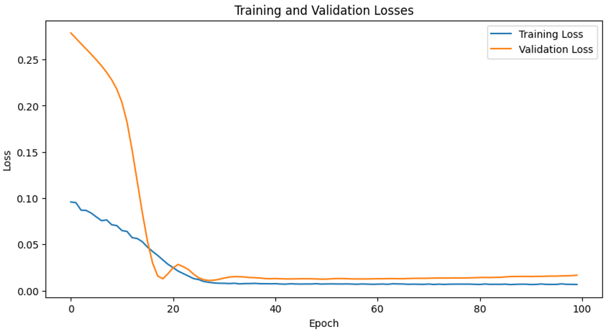
- Train the Model: Use the Adam optimizer and Huber loss function to train the model.
					# Training loop
train_losses = []
val_losses = []

for epoch in range(num_epochs):
    model.train()
    train_loss = 0
    for batch_idx, (X_batch, y_batch) in enumerate(train_loader):
        X_batch, y_batch = X_batch.to(device), y_batch.to(device)

        optimizer.zero_grad()
        outputs, _, _ = model(X_batch)
        loss = criterion(outputs, y_batch)
        loss.backward()
        optimizer.step()

        train_loss += loss.item()

        if (batch_idx + 1) % 10 == 0:
            print(f"Epoch [{epoch+1}/{num_epochs}], Batch [{batch_idx+1}/{len(train_loader)}], Train Loss: {loss.item():.4f}")

    avg_train_loss = train_loss / len(train_loader)
    train_losses.append(avg_train_loss)

    # Validation
    model.eval()
    val_loss = 0
    with torch.no_grad():
        for X_batch, y_batch in test_loader:
            X_batch, y_batch = X_batch.to(device), y_batch.to(device)
            outputs, _, _ = model(X_batch)
            val_loss += criterion(outputs, y_batch).item()

    avg_val_loss = val_loss / len(test_loader)
    val_losses.append(avg_val_loss)

    print(f"Epoch [{epoch+1}/{num_epochs}], Average Train Loss: {avg_train_loss:.4f}, Average Val Loss: {avg_val_loss:.4f}")
    print("-" * 80)
Evaluating the Model
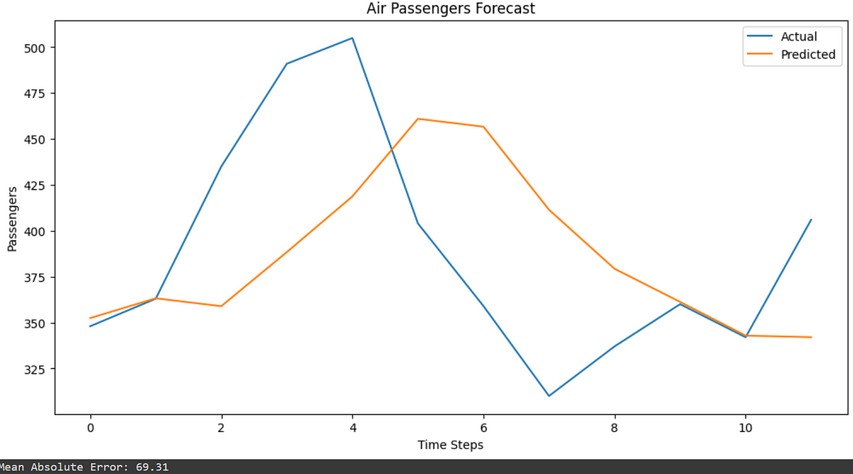
Once the training is done, we evaluate the model by comparing its predictions with actual data and calculating the Mean Absolute Error (MAE).
					# Make predictions
model.eval()
with torch.no_grad():
    X_test_tensor = torch.FloatTensor(X_test).to(device)
    predictions, _, _ = model(X_test_tensor)
    predictions = predictions.cpu().numpy()

# Inverse transform the predictions and actual values


Mathematical Intuition Behind LCN-TSF
1. Leaky Integrate-and-Fire (LIF) Neurons
LIF neurons are like little processors that handle time-based data by mimicking how biological neurons work. They:
- Have a membrane potential (think of it as their energy level).
- Receive synaptic input (external signals).
- Use decay constants to manage how quickly their energy changes over time.
- Fire (or spike) when their energy exceeds a certain threshold.
Mathematically, their energy at the next time step is:
If the energy V(t) gets too high, they spike and reset.
2. Liquid State Machine (LSM)
The LSM is a network of LIF neurons that forms a dynamic, chaotic system to process sequences over time.
- Input weights connect the input data to the neurons.
- Recurrent weights connect the neurons to each other, allowing them to influence each other over time.
This setup captures complex patterns by transforming the input and sending it through a web of neuron interactions:
3. Capsule Networks
Capsule Networks are like detailed detectives for your data. They preserve important spatial relationships and adjust themselves dynamically.
-
Squashing function: Ensures that output vectors are the right length.
-
Dynamic routing: Ensures the capsules work together effectively by updating their connections based on agreement.
4. Encoder and Decoder
-
Encoder: Combines LSM and Capsule Networks. The LSM processes the temporal (time-based) data, and the Capsule Networks refine the spatial (space-based) details.
-
Decoder: Uses an LSTM layer to turn these detailed features into predictions for future time steps.
Why LCN-TSF Rocks
So, why should you care about the Liquid Capsule Network for Time Series Forecasting (LCN-TSF)? Here are the top reasons:
- Captures Complex Patterns: LCN-TSF excels at understanding intricate and non-linear patterns in your data. Thanks to the Liquid State Machine, it’s like having a super-brain for temporal data.
- Preserves Details: With Capsule Networks, this model keeps all the tiny details intact, making sure nothing important slips through the cracks.
- Resource-Friendly: While transformers need a ton of computational power, LCN-TSF can be a more efficient choice, especially for smaller datasets or limited resources.
- Handles Long-Term Dependencies: LSMs are great at managing long-term dependencies in data, so you get a model that remembers what happened way back in your time series.
- Flexible and Powerful: Combining the strengths of spiking neurons and capsule networks, LCN-TSF is like a Swiss Army knife for time series forecasting, versatile and robust.
Comparing LCN-TSF with Transformers
Transformers have become the new stars in the world of time series forecasting. Here’s how LCN-TSF stacks up against them:
Transformers
- Self-Attention: Transformers use self-attention mechanisms to capture relationships between all time steps, making them powerful for long-term dependencies.
- Scalability: They are highly scalable and can handle large datasets efficiently.
- Complexity: Transformers are complex and require a lot of computational resources.
LCN-TSF
- Dynamic Reservoir: The LSM in LCN-TSF creates a dynamic, non-linear reservoir of spiking neurons, which is great for capturing intricate temporal patterns.
- Spatial Hierarchies: Capsule Networks in LCN-TSF preserve spatial hierarchies, making the model adept at extracting detailed features.
- Resource Efficiency: LCN-TSF, while complex, can be more resource-efficient compared to transformers, especially for smaller datasets.
Practical Takeaway
- Use Transformers if you have a large dataset and computational resources. They’re currently the state-of-the-art for many tasks.
- Try LCN-TSF if you want a model that captures complex temporal and spatial patterns efficiently, especially if you’re working with smaller datasets or have resource constraints.
Limitations of LCN-TSF
- Complexity: The architecture is pretty complicated, which can make it tough to understand and implement compared to simpler models.
- Training Time: Because it’s complex, LCN-TSF can take a while to train, especially on big datasets.
- Computational Resources: Even though it’s more efficient than transformers, it still needs a lot of computational power, especially for the LSM and capsule parts.
- Data Needs: The model performs best with a good amount of data and might not work as well with very small datasets.
- Tuning: Getting the settings right for all parts of the model (LSM, capsule layers, LSTM) can be tricky and time-consuming.
Here’s the complete code
Conclusion
The Liquid Capsule Network for Time Series Forecasting (LCN-TSF) is a powerful, innovative approach that combines the strengths of Liquid State Machines and Capsule Networks. Whether you’re tackling long-term dependencies or capturing intricate patterns, LCN-TSF offers a fresh perspective on time series forecasting. Happy forecasting!

